Step Two: Model Checking

After creating and inspecting the model in the previous Step One, we will now apply model checking to the Orchard MDP. While, strictly speaking, model checking asks whether a property holds on an MDP, we will see that modern probabilistic model checking tools, including Storm, can actually go beyond such queries. The section is structured based on the type of properties that we consider.

Preparation

We start be loading the models from the previous notebook. The complete Stormvogel model for the Orchard game is given in orchard/orchard_game_stormvogel.py. The Prism specification is given in orchard/orchard_stormvogel.pm. These models are built using functions in orchard/orchard_builder.py.

# Import stormvogel and prism models from the previous step
import stormvogel
import stormpy

from orchard.orchard_builder import build_simple, build_full, build_prism

orchard_simple = build_simple()
orchard, orchard_storm = build_full()
orchard_prism, _ = build_prism()

/__w/stormvogel/stormvogel/stormvogel/bird.py:126: UserWarning: State-action rewards are not supported in this version of stormvogel. Will assign None to the second parameter of your reward function.
  warnings.warn(

We have the following four models:

• orchard_simple is the simple Orchard game (with only two fruits) modeled in Stormvogel.

• orchard is the full Orchard game model in Stormvogel.

• orchard_storm is the orchard model in Storm data structures.

• orchard_prism is the full Orchard game model specified in the Prism modeling language.

The latter three models are semantically equivalent.

Reachability

One of the simplest properties for MDPs is a reachability query “what is the maximal probability to reach a specific set of states, described by :math:`varphi`?”. In Storm and in Stormvogel, we specify formulas in the defacto standard Prism representation, for example Pmax=? [F "Label"].

In the Orchard game, we are mostly interested in the “maximal probability of winning the game”. Using the label "PlayersWon", we express this property as Pmax=?(F "PlayersWon"), i.e. maximizing the probability of reaching a state where the players have won.

Note that, for many queries, we get a result for every state and we therefore clarify in the code that we are interested in the probability from the initial state (initial_state).

# Probability of winning the simple game
prob_players_won = 'Pmax=? [F "PlayersWon"]'
result = stormvogel.model_checking(orchard_simple, prob_players_won)
print(result.get_result_of_state(orchard_simple.initial_state))

0.5711805425946498

The resulting winning probability is \(0.5712\).

We can also visualize the result of this query on the MDP state space.

Note again that a potential warning of the form Test request failed can be safely ignored.

vis = stormvogel.show(orchard_simple, result=result)

As before, states are depicted as ellipses, actions by boxes and transitions by arrows. Labels are given inside the states and actions, and the rewards are indicated by the € symbol.

In addition, in each state, the start symbol now indicates the computed result value from that state onwards. The state is also colored with a red gradient depending on the result: the darker a state the higher its winning probability. For instance, from the state 2🍏, 1🍒, 2←🐦‍⬛, which should be visable on the right hand side (close to the initial state), the players have a winning probability of \(\frac{145}{216} = 0.671\). Following the action nextRound we can reach the successor state 🎲🐦‍⬛. Here, the probability is only \(\frac{13}{36} = 0.3611\), as the raven is then one step closer to the orchard.

The model checking also returns a memoryless policy \(\sigma\) which ensures the maximal winning probability. For each state \(s\), the policy chooses one action \(\sigma(s)\). This action is highlighted in red color in the previous Stormvogel visualization. For example, from the previous state state 2🍏, 1🍒, 2←🐦‍⬛ and action nextRound, the state 🎲🧺 is reachable. Here, the player has the option to either chooseAPPLE or to chooseCHERRY. From the red colouring, we can see that the optimal policy chooses 🍏, because the successor state has a winning probability of \(\frac{19}{24} = 0.7916\). This is higher than the non-optimal (blue colored) choice of 🍒, which only has a winning probability of \(\frac{20}{27} = 0.7407\).

For the full model orchard, the winning probability can be computed similarly.

# Probability of winning the full game
prob_players_won = 'Pmax=? [F "PlayersWon"]'
result = stormvogel.model_checking(orchard, prob_players_won)
print(result.get_result_of_state(orchard.initial_state))

0.6313570205400707

The wininng probabilty is \(0.6313\).

Total rewards

Probabilistic model checkers commonly handle reward-based queries like “what is the maximal expected total reward until reaching a specific set of states?” which can be expressed as R{rew}max=? (F "Label"), where "Label" is again describing a set of states and rew refers to the name of a reward structure.

In the Orchard game, the “maximal expected total number of rounds until the game ends” is described by R{"rounds"} max=? (F ("PlayersWon" | "RavenWon")). Here, "PlayersWon" | "RavenWon" is the disjunction of the two labels which indicate that one of the parties has won and the game has ended.

Moreover, we compute the maximal and the minimal reward. The maximal reward is achieved by a policy which maximizes the playing time, while the minimal reward corresponds to a policy minimizing the playing time.

reward_prop = 'R{"rounds"}max=? [F "PlayersWon" | "RavenWon"]'
print(
    stormvogel.model_checking(orchard, reward_prop).get_result_of_state(
        orchard.initial_state
    )
)
reward_prop = 'R{"rounds"}min=? [F "PlayersWon" | "RavenWon"]'
print(
    stormvogel.model_checking(orchard, reward_prop).get_result_of_state(
        orchard.initial_state
    )
)

22.339093430484457
20.882785206708473

Model checking reveals that the (full) game lasts between \(20.88\) and \(22.34\) rounds on average, depending on the chosen strategy of the players.

Beyond

Storm supports several queries that go significantly beyond the classical queries. While we used the Stormvogel model checking wrapper around Storm, for such properties we must often operate directly on the (somewhat more intricate) stormpy API.

We use the following helper function model_check() for simplicity. The helper function parses a property, performs the model checking on the given model for the given property and then returns the result at the initial state.

# Helper function
def model_check(model, prop):
    formula = stormpy.parse_properties(prop)[0]
    result = stormpy.model_checking(model, formula, only_initial_states=True)
    return result.at(model.initial_states[0])

Reward-bounded reachability probabilities

Reward-bounded reachability probabilities of the form Pmax=? [F{rew}<=k "Label"] ask for the probability to reach a "Label"-state while having accumulated at most \(k\) reward.

In the Orchard game, we can compute the winning probability for varying number of rounds.

# Winning probability within k rounds
probabilities = []
for k in range(41):
    win_steps = 'Pmax=? [F{"rounds"}<=' + str(k) + ' "PlayersWon"]'
    probabilities.append(model_check(orchard_prism, win_steps))
    print("Round {}: {}".format(k, probabilities[-1]))

Round 0: 0.0
Round 1: 0.0
Round 2: 0.0
Round 3: 0.0
Round 4: 0.0
Round 5: 0.0
Round 6: 0.0
Round 7: 0.0
Round 8: 0.0
Round 9: 0.0
Round 10: 0.0
Round 11: 0.0
Round 12: 0.0
Round 13: 0.0
Round 14: 0.0
Round 15: 0.0
Round 16: 0.004162126278372636
Round 17: 0.021351772506558953
Round 18: 0.060203495833722385
Round 19: 0.12409888742931646
Round 20: 0.20988036964075973
Round 21: 0.30158084132994223
Round 22: 0.3859421091236708
Round 23: 0.4560420208004474
Round 24: 0.5102170036741989
Round 25: 0.5498940328681379
Round 26: 0.5777848204667783
Round 27: 0.5967720330221457
Round 28: 0.6093722181054767
Round 29: 0.6175629247761446
Round 30: 0.6227977136574545
Round 31: 0.6260964497778784
Round 32: 0.6281506036561613
Round 33: 0.6294168505012261
Round 34: 0.6301906201480247
Round 35: 0.6306598665532833
Round 36: 0.6309425371167758
Round 37: 0.6311118037113413
Round 38: 0.6312126210507402
Round 39: 0.6312723779854957
Round 40: 0.6313076401736203

Afterwards, we can plot the results.

# Plot
import matplotlib.pyplot as plt

plt.rcParams["figure.figsize"] = (15, 5)
plt.xlabel("Number of rounds")
plt.ylabel("Probability of players winning")
plt.title("Orchard")

# Plot results for all steps
plt.plot(range(len(probabilities)), probabilities, linewidth=2)

[<matplotlib.lines.Line2D at 0x7fb3d55b6780>]

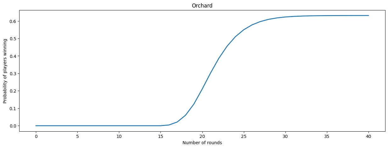
We see that the players need at least 16 rounds to win the game. For increasing number of rounds, the winning probability also increases, until it converges towards the overall winning probability of \(0.6313\).

Conditional reachability probabilities

Conditional reachability probabilities of the form Pmax=?( F "Label1" || F "Label2") express the probability of reaching a "Label1"-state, conditioned under the event that a "Label2"-state is reached.

We compute the maximal winning probability (F "PlayersWon") under the condition that the raven is eventually only one step away from the orchard (F "RavenOneAway").

Note that we use the Prism model orchard_prism here which contains additional labels such as "RavenOneAway".

print(model_check(orchard_prism, 'Pmax=? [F "PlayersWon" || F "RavenOneAway"]'))

0.3197951767821407

Checking the property yields a conditioned winning probability of \(0.3198\) which is significantly lower than the overall winning probability of \(0.6313\).

Multi-objective queries

Multi-objective queries of the form multi (formula1, ..., formulaM) allow to compute possible trade-offs between various (single-objective) properties formula1, …, formulaM.

For the Orchard game, the multi-objective query asks for the maximal expected number of rounds of the game (R{"rounds"}max=? [F ("PlayersWon" | "RavenWon")]) among all policies that induce a winning probability of at least 60% (P>=0.60 [F "PlayersWon"])).

query = (
    'multi(R{"rounds"}max=? [F ("PlayersWon" | "RavenWon")], P>=0.60 [F "PlayersWon"])'
)
print(model_check(orchard_prism, query))

21.79470309502809

We see that using a nearly optimal winning strategy (close to optimum of \(63.13\%\)) also reduces the expected number of rounds played, which is \(22.3391\) when considering all policies.